Swan Provider Income

1. Introduction

In the Swan decentralized computing ecosystem, providers earn income by executing jobs. Their income is influenced by various factors, including the number of jobs they execute, their reputation, and the Universal Basic Income (UBI) mechanism. This document outlines the mathematical model governing provider income in the Swan system.

2. Job Allocation to Nodes

Job distribution in the Swan system is done through an auction mechanism. However, the likelihood of a provider winning a job is influenced by their reputation. The job distribution engine follows a lambda distribution based on reputation scores.

Equation:

P_{win}(R) = \lambda \times e^{-\lambda R}

Where:

( P_{win}(R) ) = Probability of winning a job based on reputation ( R )
( \lambda ) = Rate parameter (determined by the system)

3. Total Jobs in the System

The total number of jobs in the system grows according to the logistic growth curve:

Equation:

Where:

( J_{total}(x) ) = Total number of jobs at time ( x )
( L_{initial} ) = Carrying capacity for initial jobs (maximum number of jobs without incentives)
( k_{initial} ) = Growth rate for initial jobs
( x_{0_{initial}} ) = Midpoint of the growth curve, where growth is fastest

4. Base Income from Jobs

Providers earn a base income from executing jobs. This income is determined by the auction mechanism, where providers bid for jobs.

Equation:

Where:

( I_{base}(j) ) = Income from job ( j )
( P_j ) = Price bid for job ( j )
( N_j ) = Number of instances of job ( j ) executed

5. Universal Basic Income (UBI)

Qualified providers receive a UBI. However, if a node has job income, the UBI is reduced by that amount. If the job income exceeds the average UBI, the UBI becomes zero.

Equation:

Where:

( I_{UBI} ) = UBI income
( U ) = Average UBI income
( I_{total_jobs} ) = Total income from all jobs

6. Bonus from Reputation

Providers with higher reputations can earn more due to a higher likelihood of winning bids in the auction system.

Equation:

Where:

( I_{bonus}(R) ) = Bonus income based on reputation ( R )

7. Total Provider Income

The total income for a provider is the sum of the base income from jobs, the UBI, and any bonuses from reputation.

Equation:

8. Conclusion

The Swan provider income model ensures a balanced distribution of income, rewarding providers for their service quality (reputation) and ensuring a safety net through the UBI. This comprehensive approach ensures the sustainability and attractiveness of the Swan ecosystem for potential providers.

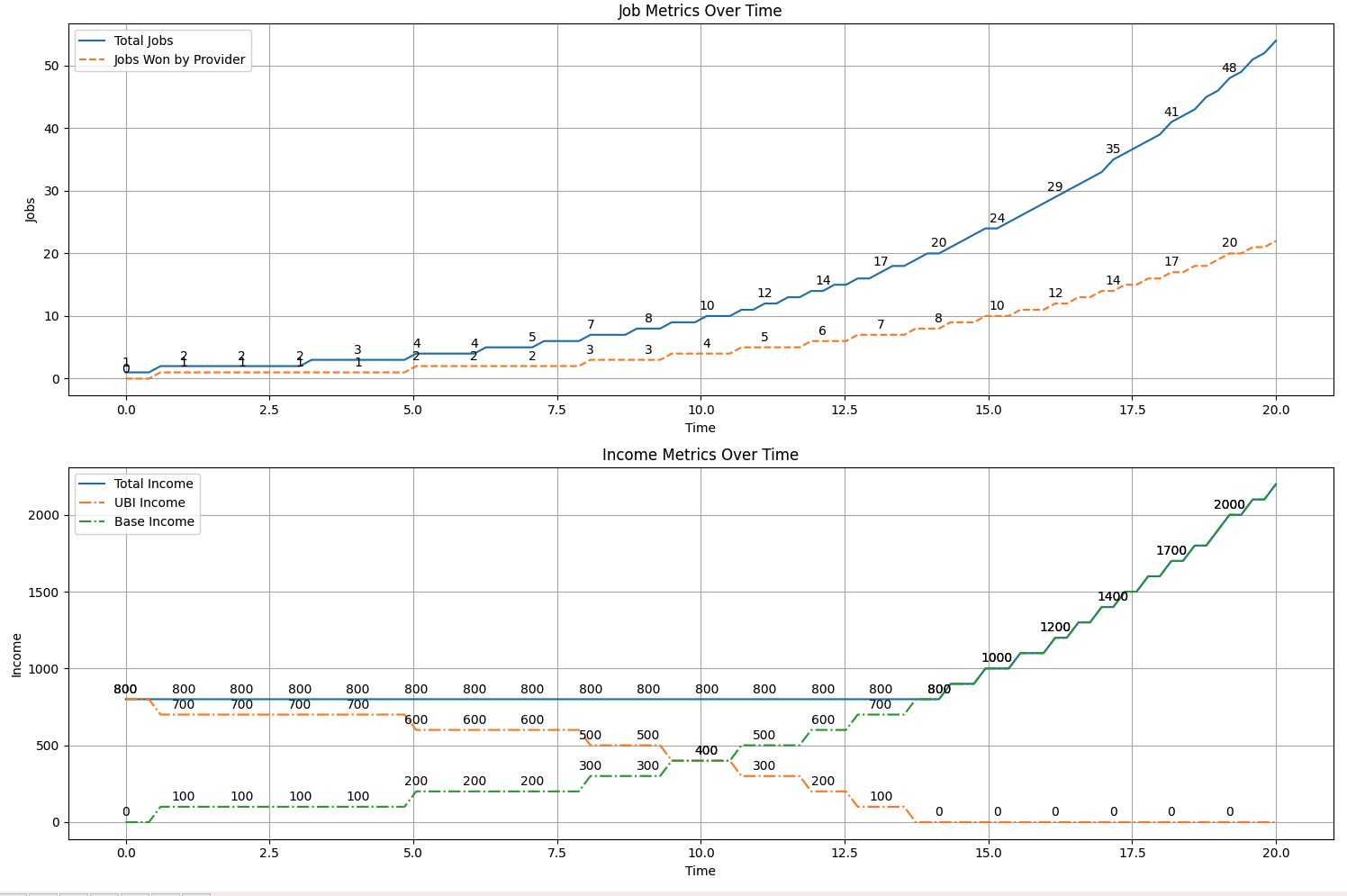
Code Simulation and Plot

import numpy as np
import matplotlib.pyplot as plt

# Parameters
lambda_parameter = 5.0
L_initial = 200
k_initial = 0.2
x_0_initial = 25
U = 800
P_j = 100  # Price bid for job

# Equations
P_win = lambda R: lambda_parameter * np.exp(-lambda_parameter * R)
J_total = lambda x: L_initial / (1 + np.exp(-k_initial * (x - x_0_initial)))
jobs_won = lambda R, total_jobs: np.round(P_win(R) * total_jobs).astype(int)
I_base = lambda jobs_won: P_j * jobs_won
I_UBI = lambda I_base: U - min(I_base, U)
I_total = lambda I_base, I_UBI: I_base + I_UBI

# Simulation
x = np.linspace(0, 20, 100)
R = 0.5  # Assuming a constant reputation score for simplicity
total_jobs = np.round(J_total(x)).astype(int)
jobs_won_by_provider = jobs_won(R, total_jobs)
base_income = I_base(jobs_won_by_provider)
ubi_income = [I_UBI(i) for i in base_income]
total_income = I_total(base_income, ubi_income)

# Plot
plt.figure(figsize=(15, 10))

# Plotting Total Jobs and Jobs Won by Provider
plt.subplot(2, 1, 1)
plt.plot(x, total_jobs, label="Total Jobs")
plt.plot(x, jobs_won_by_provider, label="Jobs Won by Provider", linestyle='--')
plt.xlabel("Time")
plt.ylabel("Jobs")
plt.title("Job Metrics Over Time")
plt.legend()
plt.grid(True)

# Annotate y-values for integer x-values
for i in range(0, len(x), 5):  # Adjusted the loop to iterate over the length of x with a step of 5
    plt.annotate(f"{total_jobs[i]}", (x[i], total_jobs[i]), textcoords="offset points", xytext=(0,5), ha='center')
    plt.annotate(f"{jobs_won_by_provider[i]}", (x[i], jobs_won_by_provider[i]), textcoords="offset points", xytext=(0,5), ha='center')

# Plotting UBI Income, Base Income, and Total Income
plt.subplot(2, 1, 2)
plt.plot(x, total_income, label="Total Income", linestyle='-')
plt.plot(x, ubi_income, label="UBI Income", linestyle='-.')
plt.plot(x, base_income, label="Base Income", linestyle='-.')
plt.xlabel("Time")
plt.ylabel("Income")
plt.title("Income Metrics Over Time")
plt.legend()
plt.grid(True)

# Annotate y-values for integer x-values
for i in range(0, len(x), 5):  # Adjusted the loop to iterate over the length of x with a step of 5
    plt.annotate(f"{total_income[i]}", (x[i], total_income[i]), textcoords="offset points", xytext=(0,5), ha='center')
    plt.annotate(f"{ubi_income[i]}", (x[i], ubi_income[i]), textcoords="offset points", xytext=(0,5), ha='center')
    plt.annotate(f"{base_income[i]}", (x[i], base_income[i]), textcoords="offset points", xytext=(0,5), ha='center')

plt.tight_layout()
plt.show()

This code simulates the provider income over time based on the equations provided. Adjust the parameters as needed to fit the specific requirements of the Swan system.

PreviousTokenomics NextGovernance

Last updated 6 months ago

import numpy as np import matplotlib.pyplot as plt # Parameters lambda_parameter = 5.0 L_initial = 200 k_initial = 0.2 x_0_initial = 25 U = 800 P_j = 100 # Price bid for job # Equations P_win = lambda R: lambda_parameter * np.exp(-lambda_parameter * R) J_total = lambda x: L_initial / (1 + np.exp(-k_initial * (x - x_0_initial))) jobs_won = lambda R, total_jobs: np.round(P_win(R) * total_jobs).astype(int) I_base = lambda jobs_won: P_j * jobs_won I_UBI = lambda I_base: U - min(I_base, U) I_total = lambda I_base, I_UBI: I_base + I_UBI # Simulation x = np.linspace(0, 20, 100) R = 0.5 # Assuming a constant reputation score for simplicity total_jobs = np.round(J_total(x)).astype(int) jobs_won_by_provider = jobs_won(R, total_jobs) base_income = I_base(jobs_won_by_provider) ubi_income = [I_UBI(i) for i in base_income] total_income = I_total(base_income, ubi_income) # Plot plt.figure(figsize=(15, 10)) # Plotting Total Jobs and Jobs Won by Provider plt.subplot(2, 1, 1) plt.plot(x, total_jobs, label="Total Jobs") plt.plot(x, jobs_won_by_provider, label="Jobs Won by Provider", linestyle='--') plt.xlabel("Time") plt.ylabel("Jobs") plt.title("Job Metrics Over Time") plt.legend() plt.grid(True) # Annotate y-values for integer x-values for i in range(0, len(x), 5): # Adjusted the loop to iterate over the length of x with a step of 5 plt.annotate(f"{total_jobs[i]}", (x[i], total_jobs[i]), textcoords="offset points", xytext=(0,5), ha='center') plt.annotate(f"{jobs_won_by_provider[i]}", (x[i], jobs_won_by_provider[i]), textcoords="offset points", xytext=(0,5), ha='center') # Plotting UBI Income, Base Income, and Total Income plt.subplot(2, 1, 2) plt.plot(x, total_income, label="Total Income", linestyle='-') plt.plot(x, ubi_income, label="UBI Income", linestyle='-.') plt.plot(x, base_income, label="Base Income", linestyle='-.') plt.xlabel("Time") plt.ylabel("Income") plt.title("Income Metrics Over Time") plt.legend() plt.grid(True) # Annotate y-values for integer x-values for i in range(0, len(x), 5): # Adjusted the loop to iterate over the length of x with a step of 5 plt.annotate(f"{total_income[i]}", (x[i], total_income[i]), textcoords="offset points", xytext=(0,5), ha='center') plt.annotate(f"{ubi_income[i]}", (x[i], ubi_income[i]), textcoords="offset points", xytext=(0,5), ha='center') plt.annotate(f"{base_income[i]}", (x[i], base_income[i]), textcoords="offset points", xytext=(0,5), ha='center') plt.tight_layout() plt.show()